These estimates often involve complex mathematical concepts and are usually presented in a highly theoretical manner (with integrals), without numerical examples explaining the calculation process. This discourages many readers who have forgotten their mathematics, as well as newcomers interested in these concepts, whether out of curiosity or because they need to understand the new requirements introduced by ISO/IEC 17025.
We will try to make these concepts more accessible through numerical examples.

Customer risk: the probability that a test or analytical result accepted by your customer is actually nonconforming.
This risk is designated by β and is expressed as probability P.
Conformity assessment body (CAB) risk (the result provider): the probability that a test or analytical result declared nonconforming is actually conforming.
This risk is designated by α and is expressed as probability P.
Let us return to our 10 pH measurements: see Decision Rules.
| 10.2 |
9.7 |
10.3 |
10.1 |
9.8 |
10.5 |
10.0 |
9.6 |
10.4 |
9.5 |
We know the upper and lower limits, the standard deviation σ = 0.348, and the expected value μ, which is simply the mean: 10.01.
The probability of obtaining conforming values is given by the following equation:

where:
The distribution is assumed to be normal (η represents the pH value).
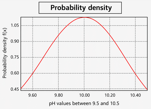
Evaluating this integral amounts to calculating the area under the Gaussian curve bounded by the limits set by the customer:

Area bounded by [9.5, 10.5].
The following Excel function calculates this area: =NORM.DIST(10.5,10.01,0.348,TRUE)-NORM.DIST(9.5,10.01,0.348,TRUE)=0.85, giving Pc = 85%.
Note that the cumulative distribution option must be TRUE.
Customer risk Rc = 1 − Pc is the difference between 100% and the probability of obtaining conforming analyses: 85%, or 15%.
Suppose my customer requires a risk Rc = 10%; Pc must therefore be 90%. I have three possible ways to reach this goal:
1) Widen the limits (by agreement with the customer).
2) Use a more precise measuring system (internal decision).
3) Keep the same equipment, narrow the acceptance limits, and account for uncertainty (internal decision).
Knowing the standard deviation of the series of measurements, we can determine a Type A uncertainty (estimated from measurement repeatability):

If I choose a guard band equal to the expanded uncertainty, assuming a normal distribution (k = 2), the limits become [9.3, 10.7].
Recalculating the area under the Gaussian curve: =NORM.DIST(10.7,10.01,0.348,TRUE)-NORM.DIST(9.3,10.01,0.348,TRUE)=0.95, giving Pc = 95%.
Customer risk Rc = 1 − Pc is the difference between 100% and the probability of obtaining conforming analyses: 95%, or 5%. The objective has been achieved.
The measuring equipment (titrator) had a 20 mL burette. I replaced it with a 5 mL burette, allowing much finer increments.
The basic pH electrode was replaced with a higher-grade electrode providing two decimal places and calibrated at three points.
My sodium hydroxide titrant, previously prepared in-house, is now purchased as a certified solution with an associated uncertainty.
Let us examine the values obtained from 10 new titrations:
| 10.16 |
9.72 |
10.25 |
10.04 |
9.84 |
10.47 |
10.00 |
9.65 |
10.36 |
9.59 |
We know the upper and lower limits, the standard deviation σ = 0.304, and the expected value μ, which is simply the mean: 10.00.
The following Excel function calculates the difference: =NORM.DIST(10.5,10.00,0.304,TRUE)-NORM.DIST(9.5,10.00,0.304,TRUE)=0.90, giving Pc = 90%.
Customer risk Rc = 1 − Pc is the difference between 100% and the probability of obtaining conforming analyses: 90%, or 10%. The objective has been achieved.
Basic assumption: the measurement series follows a normal distribution (otherwise, the function φ(z) must be expressed using another distribution).
| 10.2 |
9.7 |
10.3 |
10.1 |
9.8 |
10.5 |
10.0 |
9.6 |
10.4 |
9.5 |
The mean is y = 10.01, the standard deviation is σ = 0.348, and the Type A uncertainty is u = ±0.11.
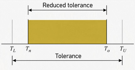
The limits are narrowed by a guard band equal to half the uncertainty, giving [T = 9.56; T = 10.44].
The customer tolerance zone is [T = 9.5; T = 10.5].
The width of the reduced interval is w = 10.44 − 9.56 = 0.88 = 4U.
Customer risk is given by the following equation:

The function φ(z) (standard normal distribution) is expressed in terms of z as follows:

F(z) is a probability function expressed as follows:

Finally, the risk of the CAB (producer) is expressed by the following equation:

Let us calculate F(z). The resulting values correspond to unrounded data.

Let us determine z, denoted z and z, as a function of the limits:

This type of function cannot generally be solved by hand and typically requires extensive numerical integration or a Monte Carlo method.
Software tools and web applications are available to help solve this type of calculation.
We will now determine R:
In fact, given the tolerance and our uncertainty, there is little reason to integrate from −∞ to +∞. Moreover, software and applications do not literally integrate these functions; they use what is known as the trapezoidal rule. The curve is divided into small bounded areas that are summed, treating each short section of the curve as approximately straight. The finer the subdivision, the better the approximation.
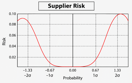
Customer risk R, calculated over [−5, −1.465] and [1.408, +5], gives 0.014, or 1.4%, well below the 10% target for a 95% probability. The objective has been achieved.
Supplier risk (CAB), calculated over [−1.465, 1.408], gives 0.086, or 8.6%, for a 95% probability, which is entirely acceptable.
A detailed calculation of this example using Excel and a mathematical method is available in the technical note “Calculating Customer and Supplier Risks with Excel.” This avoids directly calculating the integral, which is not straightforward in Excel because the Windows application cannot iteratively update the integration limits.